Multi-population LD statistics

Using moment equations for the two-locus haplotype distribution, moments.LD lets us compute a large family of linkage disequilibrium statistics in models with arbitrary mutation and recombination rates and flexible demographic history with any number of populations. The statistics are stored in a different way that the SFS, but much of the API for implementing demographic events and integration is largely consistent between the SFS and LD methods.

If you use moments.LD in your research, please cite:

[Ragsdale2019]: Ragsdale, A. P. & Gravel, S. (2019). Models of archaic admixture and recent history from two-locus statistics. PLoS Genetics, 15(6), e1008204.
[Ragsdale2020]: Ragsdale, A. P. & Gravel, S. (2020). Unbiased estimation of linkage disequilibrium from unphased data. Mol Biol Evol, 37(3), 923-932.

Linkage disequilibrium

The LD statistics that moments.LD computes are low-order summaries of expected LD between pairs of loci. In particular, we compute \(\mathbb{E}[D^2]\), the expectation of the numerator of the familiar \(r^2\) measure of LD. From this system of equations, we also compute \(\mathbb{E}[Dz] = \mathbb{E}[D(1-2p)(1-2q)]\), where \(p\) and \(q\) are the allele frequencies at the left and right loci, respectively; and we also compute \(\pi_2=\mathbb{E}[p(1-p)q(1-q)]\), a measure of the “joint heterozygosity” of the two loci [Hill1968].

These statistics are stored in a list of arrays, where each list element corresponds to a given recombination rate, \(\rho = 4N_er\), where r is the recombination probability separating loci. The length of the list is the length of the number of recombination rates given, plus one, as the last entry stores the single-locus expected heterozygosity:

import moments, moments.LD
theta = 0.001 # the mutation rate 4*Ne*u
rho = [0, 1, 10] # recombination rates 4*Ne*r between loci
y = moments.LD.Demographics1D.snm(rho=rho, theta=theta) # steady-state expectations
y

LDstats([[1.38888889e-07 1.11111111e-07 3.05555556e-07]
 [8.59375000e-08 6.25000000e-08 2.81250000e-07]
 [2.01612903e-08 8.06451613e-09 2.54032258e-07]], [0.001], num_pops=1, pop_ids=None)

Here, we can see the decay of LD with increasing recombination rate, and also that the heterozygosity equals the scaled mutation rate at steady-state, as expected. On any LD object, we can get the list of statistics present by calling:

y.names()

(['DD_0_0', 'Dz_0_0_0', 'pi2_0_0_0_0'], ['H_0_0'])

The underscores index the populations for that statistic, so DD_0_0 represents \(\mathbb{E}[D_0 D_0] = \mathbb{E}[D_0^2]\), Dz_0_0_0 represents \(\mathbb{E}[D_0(1-2p_0)(1-2q_0)]\), and pi2_0_0_0_0 represents \(\mathbb{E}[p_0(1-p_0)q_0(1-q_0)]\). Here, there is only the one population (indexed by zero), but it should be clear how the indexing extends to additional populations.

One of the great strengths of moments.LD is that while it only computes low-order moments of the full two-locus haplotype distribution, it allows us to expand the basis of statistics to include many populations. For example, one of the example demographic models for two populations is Demographics2D.split_mig, in which a single population splits into two descendant populations, each with their own relative constant sizes and connected by symmetric migration.

y = moments.LD.Demographics2D.split_mig((0.5, 2.0, 0.2, 1.0), rho=1.0)
# here, the parameters of split_mig are (T, nu0, nu1, m_sym)
print(y.names())
y

(['DD_0_0', 'DD_0_1', 'DD_1_1', 'Dz_0_0_0', 'Dz_0_0_1', 'Dz_0_1_1', 'Dz_1_0_0', 'Dz_1_0_1', 'Dz_1_1_1', 'pi2_0_0_0_0', 'pi2_0_0_0_1', 'pi2_0_0_1_1', 'pi2_0_1_0_1', 'pi2_0_1_1_1', 'pi2_1_1_1_1'], ['H_0_0', 'H_0_1', 'H_1_1'])

LDstats([[8.56755939e-08 5.27614200e-08 8.04316545e-08 7.02690405e-08
47526973e-08 5.40259243e-08 1.30708680e-07 4.83617230e-08
90151877e-08 2.29179130e-07 2.86535856e-07 2.68376752e-07
74355052e-07 3.52942478e-07 3.37909162e-07]], [0.00088908 0.00116239 0.00110805], num_pops=2, pop_ids=None)

Notice that already with just two populations we pick up many additional statistics: not just \(\mathbb{E}[D_0^2]\) and \(\mathbb{E}[D_1^2]\), but also the cross population covariance of \(D\): \(\mathbb{E}[D_0 D_1]\), as well as all possible combinations of \(D\), \(p\), and \(q\) for the Dz and pi2 moments. This is what makes such LD computation an efficient and powerful approach for inference: it is very fast to compute, it can be extended to many populations, and it gives us a large set informative statistics to compare to data and run inference.

LD decay curves

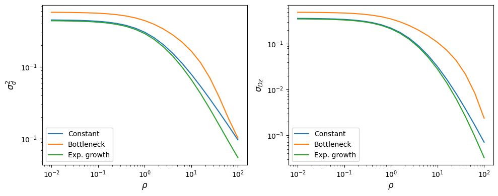
We are most often interested in examining how LD depends on recombination distances separating pairs of loci, given some underlying demography. Allele frequency correlations due to linkage are expected to break down faster with larger recombination distances, so that statistics such as \(D^2\) decrease toward zero with increasing distances between SNPs.

In the literature, we typically see the decay of \(r^2 = \mathbb{E}\left[\frac{D^2}{\pi_2}\right]\) or \(\sigma_d^2 = \frac{\mathbb{E}[D^2]}{\mathbb{E}[\pi_2]}\) reported. These are related quantities, but there is a difference between the ratio of averages and the average of ratio. While solving for \(r^2\) is very difficult, our moments framework immediately provides the expectations for \(\sigma_d^2\) and other statistics of the same form (such as what we could call \(\sigma_{Dz} = \frac{\mathbb{E}[Dz]}{\mathbb{E}[\pi_2]}\)).

Here, we’ll use demes to define a few simple models (which we’ll illustrate with demesdraw), and explore how the decay of \(\sigma_d^2\) and \(\sigma_{Dz}\) are affected by single-population demographic events. (Check out how to use Demes with moments.)

import demes, demesdraw
import matplotlib.pylab as plt

b1 = demes.Builder()
b1.add_deme(name="A", epochs=[dict(start_size=5000)])
demog_constant = b1.resolve()

b2 = demes.Builder()
b2.add_deme(
    name="A",
    epochs=[
        dict(start_size=5000, end_time=1000),
        dict(start_size=1000, end_time=400),
        dict(start_size=5000, end_time=0)
    ]
)
demog_bottleneck = b2.resolve()

b3 = demes.Builder()
b3.add_deme(
    name="A",
    epochs=[dict(start_size=5000, end_time=600), dict(end_size=10000, end_time=0)]
)
demog_growth = b3.resolve()

fig, (ax1, ax2, ax3) = plt.subplots(1, 3, figsize=(12, 4))
demesdraw.size_history(demog_constant, ax=ax1, invert_x=True)
demesdraw.size_history(demog_bottleneck, ax=ax2, invert_x=True)
demesdraw.size_history(demog_growth, ax=ax3, invert_x=True)
ax1.set_ylim(top=10000)
ax2.set_ylim(top=10000)
ax3.set_ylim(top=10000)
ax1.set_title("Constant size")
ax2.set_title("Bottleck and recovery")
ax3.set_title("Recent exponential growth");
fig.tight_layout()

For each of these models, we’ll compute LD statistics over a range of recombination rates, and then plot the decay curves.

import numpy as np

# set up recombination rates
rhos = np.logspace(-2, 2, 21)

# compute statistics and normalize to get sigma-d^2 and sigma-Dz
y_constant = moments.Demes.LD(demog_constant, sampled_demes=["A"], rho=rhos)
sigma_constant = moments.LD.Inference.sigmaD2(y_constant)

y_bottleneck = moments.Demes.LD(demog_bottleneck, sampled_demes=["A"], rho=rhos)
sigma_bottleneck = moments.LD.Inference.sigmaD2(y_bottleneck)

y_growth = moments.Demes.LD(demog_growth, sampled_demes=["A"], rho=rhos)
sigma_growth = moments.LD.Inference.sigmaD2(y_growth)

fig, (ax1, ax2) = plt.subplots(1, 2, figsize=(10, 4))

ax1.plot(rhos, sigma_constant.LD()[:, 0], label="Constant")
ax1.plot(rhos, sigma_bottleneck.LD()[:, 0], label="Bottleneck")
ax1.plot(rhos, sigma_growth.LD()[:, 0], label="Exp. growth")

ax2.plot(rhos, sigma_constant.LD()[:, 1], label="Constant")
ax2.plot(rhos, sigma_bottleneck.LD()[:, 1], label="Bottleneck")
ax2.plot(rhos, sigma_growth.LD()[:, 1], label="Exp. growth")

ax1.set_yscale("log")
ax2.set_yscale("log")
ax1.set_xscale("log")
ax2.set_xscale("log")
ax1.set_xlabel(r"$\rho$")
ax2.set_xlabel(r"$\rho$")
ax1.set_ylabel(r"$\sigma_d^2$")
ax2.set_ylabel(r"$\sigma_{Dz}$")
ax1.legend()
ax2.legend()
fig.tight_layout()

Multiple populations

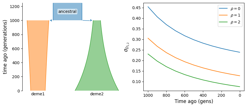
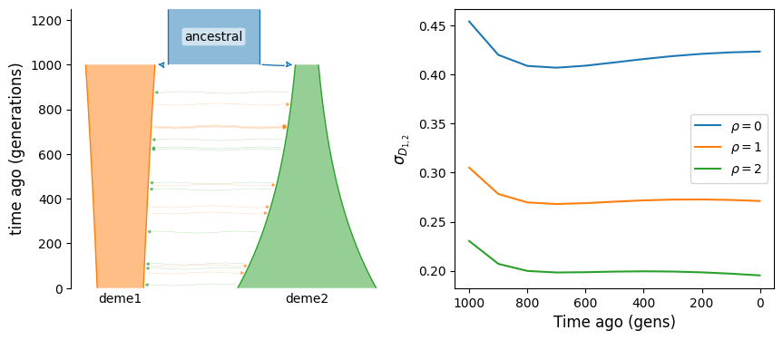
The statistic \(\mathbb{E}[D_i D_j]\), where \(i\) and \(j\) index two populations, is the covariance of LD between those populations. If these two population split from a common ancestral population, just after their split the covariance is equal to \(\mathbb{E}[D^2]\) in the ancestral population. It then decays over time, to zero if there is no migration between them and to some positive value when they are connected by ongoing migration.

Here, we consider a simple split with isolation model and compute that covariance at different times in their history.

b = demes.Builder()
b.add_deme(name="ancestral", epochs=[dict(start_size=2000, end_time=1000)])
b.add_deme(
    name="deme1",
    ancestors=["ancestral"],
    epochs=[dict(start_size=1500, end_size=1000)]
)
b.add_deme(
    name="deme2",
    ancestors=["ancestral"],
    epochs=[dict(start_size=500, end_size=3000)]
)
g = b.resolve()

# get LD stats between deme1 and deme2 and times in the past, using ancient samples
ts = np.linspace(999, 1, 11, dtype="int")
rhos = [0, 1, 2]
def get_covD(g, ts, rhos):
    covD = {rho: [] for rho in rhos}
    for t in ts:
        y = moments.Demes.LD(
            g,
            sampled_demes=["deme1", "deme2"],
            sample_times=[t, t],
            rho=rhos
        )
        for rho in rhos:
            covD[rho].append(
                moments.LD.Inference.sigmaD2(y)[rhos.index(rho)][y.names()[0].index("DD_0_1")]
            )
    return covD

covD = get_covD(g, ts, rhos)

fig, (ax1, ax2) = plt.subplots(1, 2, figsize=(10, 4))

demesdraw.tubes(g, ax=ax1)

for rho in rhos:
    ax2.plot(ts, covD[rho], label=rf"$\rho={rho}$")

ax2.invert_xaxis()
ax2.set_xlabel("Time ago (gens)")
ax2.set_ylabel(r"$\sigma_{D_{1, 2}}$")
ax2.legend();

We can see that without migration, covariance of LD across populations is expected to decay over time. If instead the two populations are connected by ongoing migration, LD will continue to have positive covariance, even long after their split from the ancestral population.

b.add_migration(demes=["deme1", "deme2"], rate=2e-3)
g = b.resolve()

covD = get_covD(g, ts, rhos)

fig, (ax1, ax2) = plt.subplots(1, 2, figsize=(10, 4))

demesdraw.tubes(g, ax=ax1)

for rho in rhos:
    ax2.plot(ts, covD[rho], label=rf"$\rho={rho}$")

ax2.invert_xaxis()
ax2.set_xlabel("Time ago (gens)")
ax2.set_ylabel(r"$\sigma_{D_{1, 2}}$")
ax2.legend();

Archaic admixture

Finally, as shown in [Ragsdale2019], the \(\sigma_{Dz}\) statistic is particularly sensitive to archaic admixture. Unlike \(\mathbb{E}[D^2]\), it is strongly elevated above single-ancestry expectations even with relatively small proportions of admixture from a deeply diverged source. Here, we have a very simple model of population that branches off from the focal population in the deep past and then provides 2% ancestry through admixture much more recently.

def admixture_model(t_pulse, prop=0.02):
    b = demes.Builder()
    b.add_deme(name="A", epochs=[dict(start_size=10000)])
    b.add_deme(
        name="B",
        ancestors=["A"],
        start_time=20000,
        epochs=[dict(start_size=2000, end_time=t_pulse)]
    )
    b.add_pulse(sources=["B"], dest="A", proportions=[prop], time=t_pulse)
    return b.resolve()

rhos = np.logspace(-2, 2, 21)

fig, (ax1, ax2, ax3) = plt.subplots(1, 3, figsize=(12, 4))

demesdraw.tubes(admixture_model(1000), ax=ax1)

# without admixture
g = admixture_model(100, prop=0)
y = moments.Demes.LD(g, sampled_demes=["A"], rho=rhos)
sigma_d2 = moments.LD.Inference.sigmaD2(y)
ax2.plot(rhos, sigma_d2.LD()[:, 0], "k--", lw=2, label="No admixture")
ax3.plot(rhos, sigma_d2.LD()[:, 1], "k--", lw=2)

# varying admixture time
for t in [1, 200, 500, 1000, 2000]:
    g = admixture_model(t)
    y = moments.Demes.LD(g, sampled_demes=["A"], rho=rhos)
    sigma_d2 = moments.LD.Inference.sigmaD2(y)
    ax2.plot(rhos, sigma_d2.LD()[:, 0], lw=1, label="$T_{pulse}=$"+f"${t}$")
    ax3.plot(rhos, sigma_d2.LD()[:, 1], lw=1)

ax2.legend()
ax2.set_xscale("log")
ax2.set_yscale("log")
ax3.set_xscale("log")
ax3.set_yscale("log")
ax2.set_xlabel(r"$\rho$")
ax3.set_xlabel(r"$\rho$")
ax2.set_ylabel(r"$\sigma_d^2$")
ax3.set_ylabel(r"$\sigma_{Dz}$")
fig.tight_layout();

Demographic events

As seen above, we can use either demes or the API to compute LD statistics under some demography. While demes is a very useful tool for building and visualizing demographic models, we sometimes want to use the built in functions to apply demographic events and integrate the LD stats object directly. Mirroring the moments API for manipulating SFS, we apply demographic events to LD objects using demographic functions that return a new LDstats object:

Extinction/marginalization

If a population goes extinct, or if we just want to stop tracking statistics involving that population, we can use y.marginalize(idx) to remove a given population or set of populations from the LD stats. Here, idx can be either an integer index or a list of integer indexes. y.marginalize() returns a new LD stats object with the specified populations removed and the population IDs preserved for the remaining populations (if given in the input LD stats).

Population splits

To split one population, we use y.split(i, new_ids=["child1", "child2"]), where i is the integer index of the population to split, and the optional argument new_ids lets us set the split population IDs. Note that if the input LD stats do not have population IDs defined (i.e y.pop_ids == None), we cannot specify new IDs.

Admixture and mergers

Admixture and merge events take two populations and combine them with given fractions of ancestry from each. The new admixed/merged population is placed at the end of the array of population indexes, and the only difference been y.admix() and y.merge() is that the merge function then removes the parental populations (i.e. the parents are marginalized after admixture).

For both functions, usage is y.admix(idx0, idx1, f, new_id="xxx"). We specify the indexes of the two parental populations (idx0 and idx1) and the proportion f contributed by the first specified population idx0 (population idx1 contributes 1-f). We can also provide the ID of the admixed population using ``new_id:

y = moments.LD.Demographics2D.snm(pop_ids=["A", "B"])
print(y.pop_ids)
y = y.admix(0, 1, 0.2, new_id="C")
print(y.pop_ids)
y = y.merge(1, 2, 0.75, new_id="D")
print(y.pop_ids)

['A', 'B']
['A', 'B', 'C']
['A', 'D']

Pulse migration

Finally, we can apply discrete (or pulse) mass migration events with a given proportion from one population to another. Here, we again specify 1) the index of the source population, 2) the index of the target/destination population, and 3) the proportion of ancestry contributed:

y = y.pulse_migrate(1, 0, 0.1)
print(y.pop_ids) # population IDs are unchanged.

['A', 'D']

Integration

Integrating the LD stats also mirrors the SFS integration function, with some changes to keyword arguments. At a minimum, we need to specify the relative sizes or size function nu and the integration time T. When simulating LD stats for one or more recombination rates, we also pass rho as a single rate or a list of rates, as needed:

y.integrate(nu, T, rho=rho, theta=theta)

For multiple populations, we can also specify a migration matrix of size \(n \times n\), where \(n\) is the number of populations that the LD stats represents. Like the SFS integration, we can also specify any populations that are frozen by passing a list of length \(n\) with True for frozen populations and False for populations to integrate.

Unlike SFS integration, LD integration also lets us specify selfing rates within each population, where selfing is a list of length \(n\) that specifies the selfing rate within each deme, which must be between 0 and 1.

References

[Hill1968]

Hill, W. G., and Alan Robertson. “Linkage disequilibrium in finite populations.” Theoretical and applied genetics 38.6 (1968): 226-231.

[Ragsdale2019] (1,2)

Ragsdale, Aaron P., and Simon Gravel. “Models of archaic admixture and recent history from two-locus statistics.” PLoS genetics 15.6 (2019): e1008204.

[Ragsdale2020]

Ragsdale, Aaron P., and Simon Gravel. “Unbiased estimation of linkage disequilibrium from unphased data.” Molecular Biology and Evolution 37.3 (2020): 923-932.