SFS Inference
Computing likelihoods
Following [Sawyer1992] the distribution of mutation frequencies is treated as a Poisson random field, so that composite likelihoods (in which we assume mutations are independent) are computed by taking Poisson likelihoods over bins in the SFS. We typically work with log-likelihoods, so that the log-likelihood of the data (\(D\)) given the model (\(M\)) is
where \(i\) indexes the bins of the SFS.
Likelihoods can be computed from moments.Inference:
import moments
import numpy as np

theta = 1000
model = theta * moments.Demographics1D.snm([10])

data = model.sample()

print(model)
print(data)
[-- 1000.0 499.9999999999999 333.33333333333326 250.0 200.0
 166.66666666666666 142.85714285714286 125.0 111.1111111111111 --]
[-- 1010 504 360 258 213 172 144 148 94 --]
print(moments.Inference.ll(model, data))
-38.19568229746642
When simulating under some demographic model, we usually use the default theta
of 1, because the SFS scales linearly in the mutation rate. When comparing to data
in this case, we need to rescale the model SFS. It turns out that the
maximum-likelihood rescaling is that which makes the total number of segregating
sites in the model equal to the total number in the data:
data = moments.Spectrum([0, 3900, 1500, 1200, 750, 720, 600, 400, 0])
model = moments.Demographics1D.two_epoch((2.0, 0.1), [8])

print("Number of segregating sites in data:", data.S())
print("Number of segregating sites in model:", model.S())
print("Ratio of segregating sites:", data.S() / model.S())

opt_theta = moments.Inference.optimal_sfs_scaling(model, data)
print("Optimal theta:", opt_theta)
Number of segregating sites in data: 9070.0
Number of segregating sites in model: 2.7771726368386327
Ratio of segregating sites: 3265.911481226729
Optimal theta: 3265.911481226729
Then we can compute the log-likelihood of the rescaled model with the data, which
will give us the same answer as moments.Inference.ll_multinom using the unscaled
data:
print(moments.Inference.ll(opt_theta * model, data))
print(moments.Inference.ll_multinom(model, data))
-59.880644681554486
-59.880644681554486
Optimization
moments optimization is effectively a wrapper for scipy optimization
routines, with some features specific to working with SFS data. In short, given
a demographic model defined by a set of parameters, we try to find those parameters
that minimize the negative log-likelihood of the data given the model. There are
a number of optimization functions available in moments.Inference:
optimizeandoptimize_log: Uses the BFGS algorithm.optimize_lbfgsbandoptimize_log_lbfgsb: Uses the L-BFGS-B algorithm.optimize_log_fmin: Uses the downhill simplex algorithm on the log of the parameters.optimize_powellandoptimize_log_powell: Uses the modified Powell’s method, which optimizes slices of parameter space sequentially.
More information about optimization algorithms can be found in the scipy documentation.
With each method, we require at least three inputs: 1) the initial guess, 2) the data SFS, and 3) the model function that returns a SFS of the same size as the data.
Additionally, it is common to set the following:
lower_boundandupper_bound: Constraints on the lower and upper bounds during optimization. These are given as lists of the same length of the parameters.fixed_params: A list of the same length of the parameters, with fixed values given matching the order of the input parameters.Noneis used to specify parameters that are still to be optimized.verbose: If an integer greater than 0, prints updates of the optimization procedure at intervals given by that spacing.
For a full description of the various inference functions, please see the SFS inference API.
Single population example
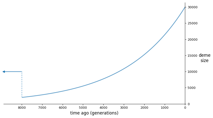
As a toy example, we’ll generate some fake data from a demographic model
and then reinfer the input parameters of that demographic model. The
model is an instantaneous bottleneck followed by exponential growth,
implemented in moments.Demographics1D.bottlegrowth, which takes
parameters [nuB, nuF, T] and the sample size. Here nuB is the
bottleneck size (relative to the ancestral size), nuF is the relative
final size, and T is the time in the past the bottleneck occurred
(in units of \(2N_e\) generations).
nuB = 0.2
nuF = 3.0
T = 0.4

n = 60  # the haploid sample size

fs = moments.Demographics1D.bottlegrowth([nuB, nuF, T], [n])

theta = 2000  # the scaled mutation rate (4*Ne*u*L)
fs = theta * fs
data = fs.sample()
The input demographic model (assuming an \(N_e\) of 10,000), plotted using demesdraw:
We then set up the optimization inputs, including the initial parameter guesses, lower bounds, and upper bounds, and then run optimization. Here, I’ve decided to use the log-L-BFGS-B method, though there are a number of built in options (see previous section).
p0 = [0.2, 3.0, 0.4]
lower_bound = [0, 0, 0]
upper_bound = [None, None, None]
p_guess = moments.Misc.perturb_params(p0, fold=1,
    lower_bound=lower_bound, upper_bound=upper_bound)

model_func = moments.Demographics1D.bottlegrowth

opt_params = moments.Inference.optimize_log_lbfgsb(
    p0, data, model_func,
    lower_bound=lower_bound,
    upper_bound=upper_bound)

model = model_func(opt_params, data.sample_sizes)
opt_theta = moments.Inference.optimal_sfs_scaling(model, data)
model = model * opt_theta
The reinferred parameters:
Params	nuB	nuF	T	theta
Input	0.2	3.0	0.4	2000
Refit	0.1529	2.555	0.4067	2.275e+03
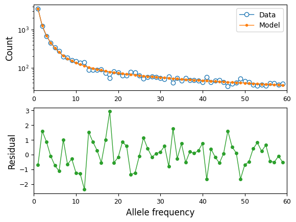
We can also visualize the fit of the model to the data:
moments.Plotting.plot_1d_comp_Poisson(model, data)
Confidence intervals
We’re often interested in estimating the precision of the inferred parameters
from our best fit model. To do this, we can compute a confidence interval for
each free parameter from the model fit. Methods implemented in moments to
compute, particularly the method based on the Godambe Information Matrix
[Coffman2016], were first implemented in dadi by Alec Coffman, who’s paper
should be cited if these methods are used.
See the API documentation for uncertainty functions for information on their usage.
Two population example
Here, we will create some fake data for a two-population split-migration model,
and then re-infer the input parameters to the model used to create that data.
This example uses the optimize_log_fmin optimization function. We’ll also
use the FIM_uncert function to compute uncertainties (reported as standard
errors).
input_theta = 10000
params = [2.0, 3.0, 0.2, 2.0]
model_func = moments.Demographics2D.split_mig
model = model_func(params, [20, 20])
model = input_theta * model
data = model.sample()

p_guess = [2, 2, .1, 4]
lower_bound = [1e-3, 1e-3, 1e-3, 1e-3]
upper_bound = [10, 10, 1, 10]

p_guess = moments.Misc.perturb_params(
    p_guess, lower_bound=lower_bound, upper_bound=upper_bound)

opt_params = moments.Inference.optimize_log_fmin(
    p_guess, data, model_func,
    lower_bound=lower_bound, upper_bound=upper_bound,
    verbose=20) # report every 20 iterations

refit_theta = moments.Inference.optimal_sfs_scaling(
    model_func(opt_params, data.sample_sizes), data)

uncerts = moments.Godambe.FIM_uncert(
    model_func, opt_params, data)

print_params = params + [input_theta]
print_opt = np.concatenate((opt_params, [refit_theta]))

print("Params\tnu1\tnu2\tT_div\tm_sym\ttheta")
print(f"Input\t" + "\t".join([str(p) for p in print_params]))
print(f"Refit\t" + "\t".join([f"{p:.4}" for p in print_opt]))
print(f"Std-err\t" + "\t".join([f"{u:.3}" for u in uncerts]))

moments.Plotting.plot_2d_comp_multinom(
    model_func(opt_params, data.sample_sizes), data)
120 , -1899.6 , array([ 2.13997 , 2.38495 , 0.276117 , 4.0609 ])
140 , -1372.36 , array([ 1.78908 , 2.57159 , 0.226001 , 1.84622 ])
160 , -1297.03 , array([ 1.79766 , 2.70804 , 0.264754 , 2.46429 ])
180 , -1217.72 , array([ 1.9792 , 2.95772 , 0.185747 , 2.07648 ])
200 , -1208.23 , array([ 1.96166 , 2.96064 , 0.19517 , 2.00892 ])
220 , -1208.03 , array([ 1.94762 , 2.95467 , 0.196843 , 2.03397 ])
240 , -1208.01 , array([ 1.93962 , 2.95089 , 0.197167 , 2.04576 ])
260 , -1208.01 , array([ 1.942 , 2.95435 , 0.197296 , 2.04196 ])
Params	nu1	nu2	T_div	m_sym	theta
Input	2.0	3.0	0.2	2.0	10000
Refit	1.942	2.954	0.1973	2.042	1.014e+04
Std-err	0.0381	0.0653	0.00435	0.0722	70.1
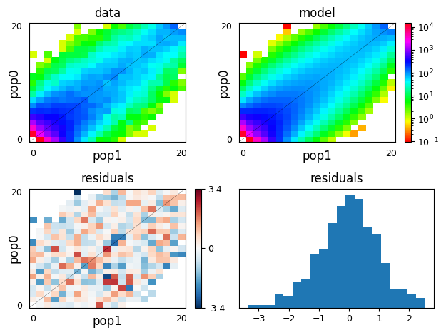
Above, we can see that we recovered the parameters used to simulate the data
very closely, and we used moments’s plotting features to visually compare
the data to the model fit.
References
Sawyer, Stanley A., and Daniel L. Hartl. “Population genetics of polymorphism and divergence.” Genetics 132.4 (1992): 1161-1176.
Coffman, Alec J., et al. “Computationally efficient composite likelihood statistics for demographic inference.” Molecular biology and evolution 33.2 (2016): 591-593.