Demography and genetic diversity
Todo
This module has not been completed.
Intro - intuition about how demography is expected to affect summary statistics helps in hypothesizing historical scenarios to explain observed patterns of genetic diversity, or trouble-shooting poor fits of models to data. It’s also important to understand how demographic parameters can be confounded and different evolutionary scenarios can give rise to similar patterns of genetic diversity.
Measures of genetic diversity
Many of the common single-site diversity statistics we are familiar with in population genetics are summaries of the SFS.
For single populations, diversity within a population is very often reported as the average heterozygosity (typically denoted \(\pi\) or \(H\)): the probability that two genome copies (i.e. samples) differ in state at a given locus. Suppose our SFS stores the distribution of allele frequencies over \(L\) loci for \(n\) samples. Then the expected or average \(\pi\) can be found by summing across allele frequency bins in the SFS and computing the probability that two randomly drawn copies carry different alleles for the given allele frequency:
Under the standard neutral model with steady-state demography, diversity is expected to be equal to the scaled mutation rate:
import moments

theta = 0.001 # the per-base scaled mutation rate, 4*Ne*u
n = 30 # the haploid sample size
fs = theta * moments.Demographics1D.snm([n])

print("Theta:", theta)
print("Diversity:", f"{fs.pi():0.4f}")
Theta: 0.001
Diversity: 0.0010
Single-population demography
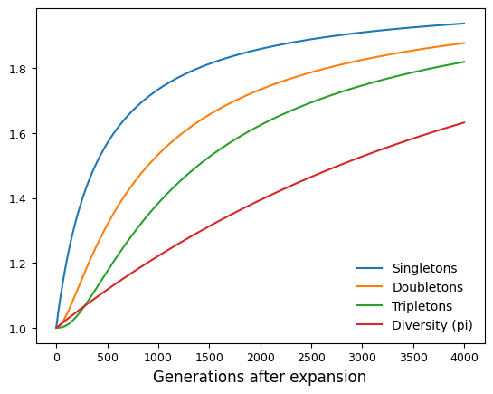
Store values every x generations after instantaneouls double of size:
Ne = 1000

singletons = []
doubletons = []
tripletons = []
diversity = []

fs = moments.Demographics1D.snm([20])
singletons.append(fs[1])
doubletons.append(fs[2])
tripletons.append(fs[3])
diversity.append(fs.pi())

for gens in range(Ne):
    fs.integrate([2], 4/2/Ne)
    singletons.append(fs[1])
    doubletons.append(fs[2])
    tripletons.append(fs[3])
    diversity.append(fs.pi())

import matplotlib.pylab as plt
fig = plt.figure(1)
ax = plt.subplot(1, 1, 1)
tt = [4 * t for t in range(Ne + 1)]
ax.plot(tt, singletons / singletons[0], label="Singletons")
ax.plot(tt, doubletons / doubletons[0], label="Doubletons")
ax.plot(tt, tripletons / tripletons[0], label="Tripletons")
ax.plot(tt, diversity / diversity[0], label="Diversity (pi)")
ax.set_xlabel("Generations after expansion")
ax.legend(frameon=False)
<matplotlib.legend.Legend at 0x7f8b8379fcb0>

Tajima’s D and pi over time with size changes
dynamics of allele frequency classes with size changes
Multiple populations
Comparison to some classical result in an IM model?
m-T confounding in heatmap of Fst
Fst with small sizes vs large divergence
pi over time in OOA model