DFE inference
By Aaron Ragsdale, November 2020.
The distribution of fitness effects (DFE) for new mutations describes is a fundamental parameter in evolutionary biology - it determines the fixation probability of new functional mutations, the strength of background selection, and the genetic architecture of traits and disease.
Very roughly, most new mutations across the genome are effectively neutral or deleterious, with a small fraction being beneficial (e.g. [Keightley], [Boyko]). In coding regions, the average selection coefficient for a new mutation depends on its functional effect: we typically assume synonymous (or silent) mutations are effectively neutral (though this may be a tenuous assumption!), missense (or nonsynonymous) mutations are more deleterious on average, and loss-of-function (or nonsense) mutations are often very damaging. We can learn about the DFE in each of these categories by studying the distributions allele frequencies for variants in each class.
Data
Let’s first look at the data we’ll be working with. Here, I used single-population data from the Mende from Sierre Leone (MSL) from the 1000 Genomes Project [1000G]. In Fig. 2, I plotted the unfolded SFS for three classes of mutations in coding regions genome-wide. We can see that the missense variants are skewed to lower frequencies than synonymous variants, on average, and loss-of-function (LOF) variants are skewed to even lower frequencies.
It can be difficult to judge the skew of the SFS based on SFS counts, since the total mutational target for each mutation class differs (Table 1). In the bottom panel of the plot, we can see that of all LOF variants observed in the MSL population, roughly 50% of them are singletons; compare that to synonymous variants, of which less than 30% are singletons.
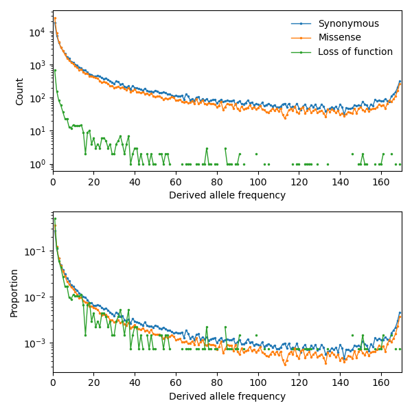
Fig. 2 Synonymous, missense, and loss-of-function SFS from the 1000 Genomes Project across all autosomal genes. Top: counts in each frequency bin. Bottom: proportions in each frequency bin.
Mutation rates
The overall scaling of the SFS from mutation classes is also informative, because strongly deleterious or lethal mutations are quickly lost from the population and so are often unseen. Thus, seeing fewer mutations that expected in a given class tells us that some fraction of those mutations are highly deleterious. To make such an inference about the strongly damaging tail fo the DFE we need to know the total mutation rates for each class of mutations.
Using the mutation model from [Karczewski], I summed across all possible mutations in
genes genome-wide, their mutational probability, and their functional consequences to
get the total mutation rate (u*L - here, L is roughly 36 Mb of annotated coding
regions) for each of the three mutation classes shown in Fig. 2:
Mutation class |
Total mutation rate |
Synonymous variants |
0.1442 |
Missense variants |
0.3426 |
Loss-of-function variants |
0.0256 |
We can see here that the mutational target for nonsynonymous variants is about 2.37 times larger than for synonymous variants. Still, we see far more segregating synonymous mutations than nonsynonymous mutations:
import moments
import pickle
import numpy as np

# note that these frequency spectra are saved in the docs directory of the moments
# repository: https://github.com/MomentsLD/moments/tree/main/docs/data
data = pickle.load(open("./data/msl_data.bp", "rb"))

fs_syn = data["spectra"]["syn"]
fs_mis = data["spectra"]["mis"]
fs_lof = data["spectra"]["lof"]

u_syn = data["rates"]["syn"]
u_mis = data["rates"]["mis"]
u_lof = data["rates"]["lof"]

print("Diversity:")
print(f"synonymous:\t{fs_syn.pi():.2f}")
print(f"missense:\t{fs_mis.pi():.2f}")
print(f"loss of func:\t{fs_lof.pi():.2f}")

print()
print("Diversity scaled by total mutation rate:")
print(f"synonymous:\t{fs_syn.pi() / u_syn:.2f}")
print(f"missense:\t{fs_mis.pi() / u_mis:.2f}")
print(f"loss of func:\t{fs_lof.pi() / u_lof:.2f}")
Diversity:
synonymous:	8452.01
missense:	6991.16
loss of func:	95.16

Diversity scaled by total mutation rate:
synonymous:	58614.15
missense:	20408.81
loss of func:	3718.19
Controlling for demography
Demography (in this case, the population size history) affects mutation frequency trajectories and the SFS, so we need to control for non-steady-state demography in some way. Using our assumption that synonymous variants are effectively neutral, we first fit a demographic model to synonymous variants, and then with that inferred demography we fit the DFE to selected variants.
We could pick any plausible demographic model to fit. The main consideration is to choose a demographic model that can adequately fit the data, but is not so over-parameterized to be overfitting to the noise in the SFS. In Fig. 2, we can also see the telltale sign of ancestral misidentification by the uptick of high-frequency variants. In addition to the demographic parameters (sizes and epoch times), we wil also fit a parameter to account for the probability of mis-polarizing a variant.
Let’s fit a model with three epochs: the ancestral size, an ancient expansion, and a
recent exponential growth. In fitting the demography, we keep multinom=True, the
default, as we don’t have an estimate for \(N_e\).
def model_func(params, ns):
    nuA, nuF, TA, TF, p_misid = params
    fs = moments.Demographics1D.snm(ns)
    fs.integrate([nuA], TA)
    nu_func = lambda t: [nuA * np.exp(np.log(nuF / nuA) * t / TF)]
    fs.integrate(nu_func, TF)
    fs = (1 - p_misid) * fs + p_misid * fs[::-1]
    return fs

p_guess = [2.0, 10.0, 0.3, 0.01, 0.02]
lower_bound = [1e-3, 1e-3, 1e-3, 1e-3, 1e-3]
upper_bound = [10, 100, 1, 1, 0.999]

opt_params = moments.Inference.optimize_log_fmin(
    p_guess, fs_syn, model_func,
    lower_bound=lower_bound, upper_bound=upper_bound)

model = model_func(opt_params, fs_syn.sample_sizes)
opt_theta = moments.Inference.optimal_sfs_scaling(model, fs_syn)
Ne = opt_theta / u_syn / 4

print("optimal demog. parameters:", opt_params[:-1])
print("anc misid:", opt_params[-1])
print("inferred Ne:", f"{Ne:.2f}")
optimal demog. parameters: [2.21531687 5.29769918 0.55450117 0.04088086]
anc misid: 0.01975812
inferred Ne: 11372.91
Log-likelihood: -689.7426549382199
Note that I initialized the model parameters fairly close to the optimal parameters. In practice, you would want to test a wide range of initial conditions to make sure our inference didn’t get stuck at a local minimum.
We can see how well our model fit the synonymous data:
moments.Plotting.plot_1d_comp_multinom(model, fs_syn, residual="linear")

# Demographic model fit to the MSL synonymous data. Top: model (red) and synonymous
# data (blue) SFS. Bottom: residuals, plotted as ``(model - data) / sqrt(data)``.
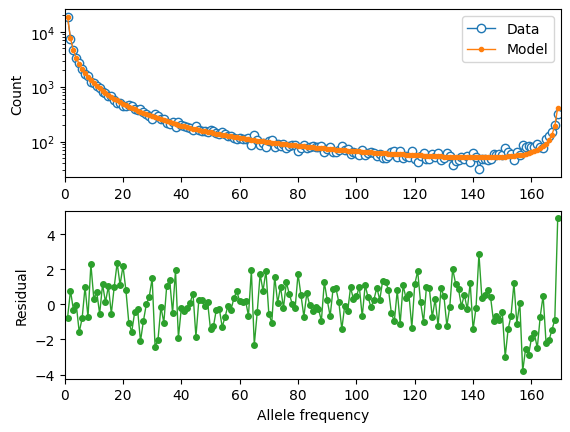
That’s a pretty good fit! Now that we have our inferred demographic model, let’s move on to inferring the DFEs for missense and LOF variants.
Inferring the DFE
Now that we have a plausible demographic model, we can move to the selected SFS. Not every new missense mutation or every new LOF mutation will have the same fitness effect, so we aim to learn the distribution of selection coefficients of new mutations. Here, we are going to assume an additive model of selection - that is, heterozygotes have fitness \(1+s\) while homozygotes for the derived allele have fitness \(1+2s\). We’re also only going to focus on the deleterious DFE - we assume beneficial mutations are very rare, and we’ll ignore them.
The general strategy is to pick some distribution (here, we’ll choose a gamma distribution, though other distributions such a log-normal or point masses could be used), and then infer the parameters of that distribution. To do so, we compute a large number of SFS spanning the range of the distribution of possible \(\gamma=2N_es\) values, and then combine them based on weights given by the parameterized DFE (for example, [Ragsdale], [Kim]).
Because the underlying demographic model does not change, we can cache the SFS for each value of \(\gamma\). Then in optimizing the DFE parameters, we just have a weighted sum across this cache, and this makes the actual DFE inference very rapid.
Caching SFS
We cache the SFS for the inferred demography and a grid of selection coefficients ranging from neutral to strongly deleterious. For the SFS with very deleterious selection coefficients, the computation is only stable with large sample sizes. Thus, after each computation for a given selection coefficient, we check to make sure that the SFS does not have large negative oscillations and did not fail to converge. If the computation failed, we doube the sample size and recompute the SFS, repeating until we have a sample size large enough to stably compute the SFS. That SFS is then projected to the needed sample size and chached.
def selection_spectrum(gamma, h=0.5):
    rerun = True
    ns_sim = 100
    while rerun:
        ns_sim = 2 * ns_sim
        fs = moments.LinearSystem_1D.steady_state_1D(ns_sim, gamma=gamma, h=h)
        fs = moments.Spectrum(fs)
        fs.integrate([opt_params[0]], opt_params[2], gamma=gamma, h=h)
        nu_func = lambda t: [opt_params[0] * np.exp(
            np.log(opt_params[1] / opt_params[0]) * t / opt_params[3])]
        fs.integrate(nu_func, opt_params[3], gamma=gamma, h=h)
        if abs(np.max(fs)) > 10 or np.any(np.isnan(fs)):
            # large gamma-values can require large sample sizes for stability
            rerun = True
        else:
            rerun = False
    fs = fs.project(fs_syn.sample_sizes)
    return fs

spectrum_cache = {}
spectrum_cache[0] = selection_spectrum(0)

gammas = np.logspace(-4, 3, 61)
for gamma in gammas:
    spectrum_cache[gamma] = selection_spectrum(-gamma)
Optimization of the DFE
We’ll fit a gamma distribution for the DFE, which has parameters alpha and beta. First, we set up the expected thetas for both missense and LOF mutations, as well as the function that weights the cached spectra based on the gamma distribution. The parameters we fit are then alpha and beta (or shape and scale) of the gamma distribution and the misidentification rate.
import scipy.stats
theta_mis = opt_theta * u_mis / u_syn
theta_lof = opt_theta * u_lof / u_syn

dxs = ((gammas - np.concatenate(([gammas[0]], gammas))[:-1]) / 2
    + (np.concatenate((gammas, [gammas[-1]]))[1:] - gammas) / 2)

def dfe_func(params, ns, theta=1):
    alpha, beta, p_misid = params
    fs = spectrum_cache[0] * scipy.stats.gamma.cdf(gammas[0], alpha, scale=beta)
    weights = scipy.stats.gamma.pdf(gammas, alpha, scale=beta)
    for gamma, dx, w in zip(gammas, dxs, weights):
        fs += spectrum_cache[gamma] * dx * w
    fs = theta * fs
    return (1 - p_misid) * fs + p_misid * fs[::-1]

def model_func_missense(params, ns):
    return dfe_func(params, ns, theta=theta_mis)

def model_func_lof(params, ns):
    return dfe_func(params, ns, theta=theta_lof)
Fit missense variants:
p_guess = [0.2, 1000, 0.01]
lower_bound = [1e-4, 1e-1, 1e-3]
upper_bound = [1e1, 1e5, 0.999]

opt_params_mis = moments.Inference.optimize_log_fmin(
    p_guess, fs_mis, model_func_missense,
    lower_bound=lower_bound, upper_bound=upper_bound,
    multinom=False)

model_mis = model_func_missense(opt_params_mis, fs_mis.sample_sizes)
print("optimal parameters:")
print("shape:", f"{opt_params_mis[0]:.4f}")
print("scale:", f"{opt_params_mis[1]:.1f}")
print("anc misid:", f"{opt_params_mis[2]:.4f}")
print("Log-likelihood:", moments.Inference.ll_multinom(model_mis, fs_mis))
optimal parameters:
shape: 0.1596
scale: 2332.3
anc misid: 0.0137
Log-likelihood: -695.1273435550039
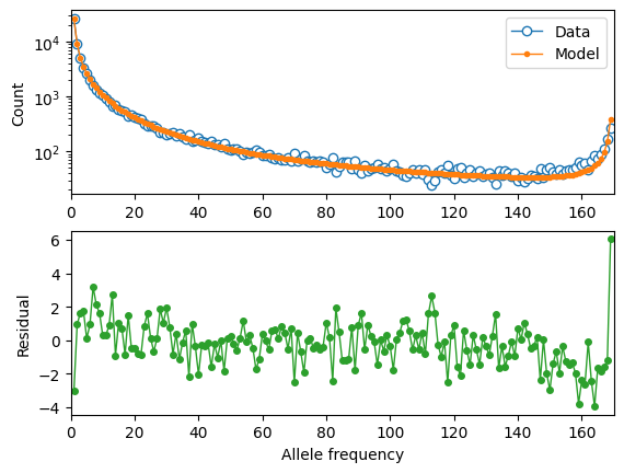
To visualize the fit of our inferred model to the missense data:
moments.Plotting.plot_1d_comp_Poisson(model_mis, fs_mis, residual="linear")

# Gamma-DFE fit to the MSL missense data.
Next, we fit LOF variants in exactly the same way:
p_guess = [0.2, 1000, 0.01]
lower_bound = [1e-4, 1e-1, 1e-3]
upper_bound = [1e1, 1e5, 0.999]

opt_params_lof = moments.Inference.optimize_log_fmin(
    p_guess, fs_lof, model_func_lof,
    lower_bound=lower_bound, upper_bound=upper_bound,
    multinom=False)

model_lof = model_func_lof(opt_params_lof, fs_lof.sample_sizes)
print("optimal parameters:")
print("shape:", f"{opt_params_lof[0]:.4f}")
print("scale:", f"{opt_params_lof[1]:.1f}")
print("anc misid:", f"{opt_params_lof[2]:.4f}")
print("Log-likelihood:", moments.Inference.ll_multinom(model_lof, fs_lof))
optimal parameters:
shape: 0.3589
scale: 7830.5
anc misid: 0.0021
Log-likelihood: -232.5947964981528
optimal parameters:
shape: 0.3589
scale: 7830.5
anc misid: 0.0021
Log-likelihood: -232.59479649929824
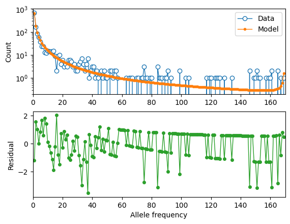
And again we visualize the fit of our inferred model to the LOF data:
moments.Plotting.plot_1d_comp_Poisson(model_lof, fs_lof, residual="linear")

# Gamma-DFE fit to the MSL loss-of-function data.
Using the inferred \(N_e\) from fitting the demographic model to the synonymous
data and the function scipy.stats.gamma.cdf(), we can compute the proportions
of new missense and LOF mutations across bins of selection coefficients:
Class |
\(| s | < 10^{-5}\) |
\(10^{-5} \leq | s | < 10^{-4}\) |
\(10^{-4} \leq | s | < 10^{-3}\) |
\(10^{-3} \leq | s | < 10^{-2}\) |
\(| s | \geq 10^{-2}\) |
Missense |
0.246 |
0.109 |
0.157 |
0.219 |
0.268 |
LOF |
0.026 |
0.034 |
0.078 |
0.175 |
0.687 |
Here, we clearly see that LOF variants are inferred to be very deleterious, with roughly 2/3 of all new LOF mutations having a selection coefficient larger that \(10^{-2}\).
Sensitivity to the demographic model
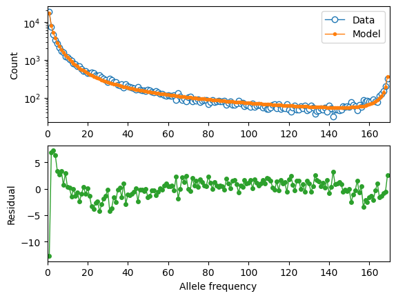
Here, we’ll fit a simpler models to the synonymous variants, and rerun the same DFE inference to check if the results are robust. We’ll first fit a two-epoch model (again accounting for ancestral misidentification), and then simply use a standard neutral model without size changes.
Throughout this section, we again print log-likelihoods of the fits, which can be compared to the fits made with the more complex demographic model above.
def model_func(params, ns):
    nu, T, p_misid = params
    fs = moments.Demographics1D.two_epoch([nu, T], ns)
    fs = (1 - p_misid) * fs + p_misid * fs[::-1]
    return fs

p_guess = [2, .3, 0.02]
lower_bound = [1e-3, 1e-3, 1e-3]
upper_bound = [10, 1, 0.999]

opt_params = moments.Inference.optimize_log_fmin(
    p_guess, fs_syn, model_func,
    lower_bound=lower_bound, upper_bound=upper_bound)

model = model_func(opt_params, fs_syn.sample_sizes)
opt_theta = moments.Inference.optimal_sfs_scaling(model, fs_syn)
Ne = opt_theta / u_syn / 4

print("optimal demog. parameters:", opt_params[:-1])
print("anc misid:", opt_params[-1])
print("inferred Ne:", f"{Ne:.2f}")
print("Log-likelihood:", moments.Inference.ll_multinom(model, fs_syn))
# compare log-likelihood to the more complex demographic model above

moments.Plotting.plot_1d_comp_multinom(model, fs_syn, residual="linear")
optimal demog. parameters: [2.55501781 0.31744642]
anc misid: 0.01842965
inferred Ne: 12518.37
Log-likelihood: -908.8631695023321
Now we cache the selection-SFS for this demography and refit the DFE to the missense variants:
def selection_spectrum(gamma):
    rerun = True
    ns_sim = 100
    while rerun:
        ns_sim = 2 * ns_sim
        fs = moments.LinearSystem_1D.steady_state_1D(ns_sim, gamma=gamma)
        fs = moments.Spectrum(fs)
        fs.integrate([opt_params[0]], opt_params[1], gamma=gamma)
        if abs(np.max(fs)) > 10 or np.any(np.isnan(fs)):
            # large gamma-values can require large sample sizes for stability
            rerun = True
        else:
            rerun = False
    fs = fs.project(fs_syn.sample_sizes)
    return fs

spectrum_cache = {}
spectrum_cache[0] = selection_spectrum(0)

gammas = np.logspace(-4, 3, 61)
for gamma in gammas:
    spectrum_cache[gamma] = selection_spectrum(-gamma)
Set up the mutation rates and DFE functions:
theta_mis = opt_theta * u_mis / u_syn
theta_lof = opt_theta * u_lof / u_syn

dxs = ((gammas - np.concatenate(([gammas[0]], gammas))[:-1]) / 2
    + (np.concatenate((gammas, [gammas[-1]]))[1:] - gammas) / 2)

def dfe_func(params, ns, theta=1):
    alpha, beta, p_misid = params
    fs = spectrum_cache[0] * scipy.stats.gamma.cdf(gammas[0], alpha, scale=beta)
    weights = scipy.stats.gamma.pdf(gammas, alpha, scale=beta)
    for gamma, dx, w in zip(gammas, dxs, weights):
        fs += spectrum_cache[gamma] * dx * w
    fs = theta * fs
    return (1 - p_misid) * fs + p_misid * fs[::-1]

def model_func_missense(params, ns):
    return dfe_func(params, ns, theta=theta_mis)

def model_func_lof(params, ns):
    return dfe_func(params, ns, theta=theta_lof)
Fit the missense data:
p_guess = [0.2, 1000, 0.01]
lower_bound = [1e-4, 1e-1, 1e-3]
upper_bound = [1e1, 1e5, 0.999]

opt_params_mis = moments.Inference.optimize_log_fmin(
    p_guess, fs_mis, model_func_missense,
    lower_bound=lower_bound, upper_bound=upper_bound,
    multinom=False)

model_mis = model_func_missense(opt_params_mis, fs_mis.sample_sizes)
print("optimal parameters (missense):")
print("shape:", f"{opt_params_mis[0]:.4f}")
print("scale:", f"{opt_params_mis[1]:.1f}")
print("anc misid:", f"{opt_params_mis[2]:.4f}")
print("Log-likelihood:", moments.Inference.ll_multinom(model_mis, fs_mis))

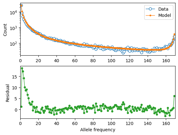
moments.Plotting.plot_1d_comp_Poisson(model_mis, fs_mis, residual="linear")
optimal parameters (missense):
shape: 0.1830
scale: 733.6
anc misid: 0.0134
Log-likelihood: -999.0833946058096
Fit the LOF data:
p_guess = [0.2, 1000, 0.01]
lower_bound = [1e-4, 1e-1, 1e-3]
upper_bound = [1e1, 1e5, 0.999]

opt_params_lof = moments.Inference.optimize_log_fmin(
    p_guess, fs_lof, model_func_lof,
    lower_bound=lower_bound, upper_bound=upper_bound,
    multinom=False)

model_lof = model_func_lof(opt_params_lof, fs_lof.sample_sizes)
print("optimal parameters:")
print("shape:", f"{opt_params_lof[0]:.4f}")
print("scale:", f"{opt_params_lof[1]:.1f}")
print("anc misid:", f"{opt_params_lof[2]:.4f}")
print("Log-likelihood:", moments.Inference.ll_multinom(model_lof, fs_lof))

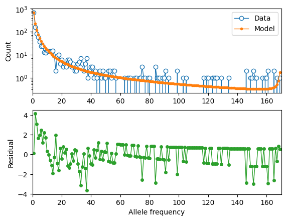
moments.Plotting.plot_1d_comp_Poisson(model_lof, fs_lof, residual="linear")
optimal parameters:
shape: 0.3937
scale: 3802.9
anc misid: 0.0021
Log-likelihood: -246.78811141192315
We can compare our results using this simpler two-epoch demographic model to our previous findings:
print("Missense DFE:")
shape = opt_params_mis[0]
scale = opt_params_mis[1]
ss = [0, 1e-5, 1e-4, 1e-3, 1e-2]
for s0, s1 in zip(ss[:-1], ss[1:]):
    cdf0 = scipy.stats.gamma.cdf(2 * Ne * s0, shape, scale=scale)
    cdf1 = scipy.stats.gamma.cdf(2 * Ne * s1, shape, scale=scale)
    print(f"{s0} <= s < {s1}:", f"{cdf1 - cdf0:.3f}")
    if s1 == ss[-1]:
        print(f"s >= {s1}:", f"{1 - cdf1:.3f}")

print()
print("LOF DFE:")
shape = opt_params_lof[0]
scale = opt_params_lof[1]
ss = [0, 1e-5, 1e-4, 1e-3, 1e-2]
for s0, s1 in zip(ss[:-1], ss[1:]):
    cdf0 = scipy.stats.gamma.cdf(2 * Ne * s0, shape, scale=scale)
    cdf1 = scipy.stats.gamma.cdf(2 * Ne * s1, shape, scale=scale)
    print(f"{s0} <= s < {s1}:", f"{cdf1 - cdf0:.3f}")
    if s1 == ss[-1]:
        print(f"s >= {s1}:", f"{1 - cdf1:1.3f}")
Missense DFE:
0 <= s < 1e-05: 0.251
1e-05 <= s < 0.0001: 0.132
0.0001 <= s < 0.001: 0.198
0.001 <= s < 0.01: 0.266
s >= 0.01: 0.153

LOF DFE:
0 <= s < 1e-05: 0.025
1e-05 <= s < 0.0001: 0.038
0.0001 <= s < 0.001: 0.093
0.001 <= s < 0.01: 0.223
s >= 0.01: 0.621
Comparing to the table above, these look pretty similar - that’s a good sign that our inferences are fairly robust to slightly poorer fits of the demographic model.
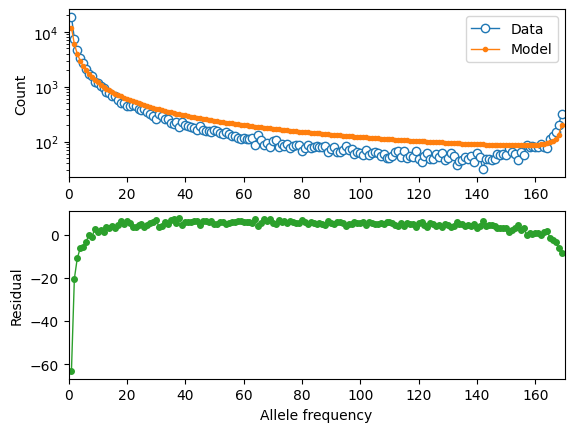
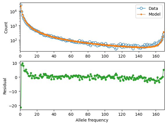
But what if our demographic model is way off, such as assuming constant population size?
# here, we'll only fit the ancestral-state misidentification rate
def model_func(params, ns):
    p_misid = params
    fs = moments.Demographics1D.snm(ns)
    fs = (1 - p_misid) * fs + p_misid * fs[::-1]
    return fs

p_guess = [0.02]
lower_bound = [1e-3]
upper_bound = [0.999]

opt_params = moments.Inference.optimize_log_fmin(
    p_guess, fs_syn, model_func,
    lower_bound=lower_bound, upper_bound=upper_bound)

model = model_func(opt_params, fs_syn.sample_sizes)
opt_theta = moments.Inference.optimal_sfs_scaling(model, fs_syn)
Ne = opt_theta / u_syn / 4

print("optimal Ne scaling:", f"{Ne:.2f}")
print("Log-likelihood:", moments.Inference.ll_multinom(model, fs_syn))

moments.Plotting.plot_1d_comp_multinom(model, fs_syn, residual="linear")
optimal Ne scaling: 20930.55
Log-likelihood: -4856.9252040098
Set up the spectrum cache for this constant-size demographic model:
def selection_spectrum(gamma):
    fs = moments.LinearSystem_1D.steady_state_1D(fs_syn.sample_sizes[0], gamma=gamma)
    fs = moments.Spectrum(fs)
    return fs

spectrum_cache = {}
spectrum_cache[0] = selection_spectrum(0)

gammas = np.logspace(-4, 3, 61)
for gamma in gammas:
    spectrum_cache[gamma] = selection_spectrum(-gamma)
Set up the mutation rates and DFE functions:
theta_mis = opt_theta * u_mis / u_syn
theta_lof = opt_theta * u_lof / u_syn

dxs = ((gammas - np.concatenate(([gammas[0]], gammas))[:-1]) / 2
    + (np.concatenate((gammas, [gammas[-1]]))[1:] - gammas) / 2)

def dfe_func(params, ns, theta=1):
    alpha, beta, p_misid = params
    fs = spectrum_cache[0] * scipy.stats.gamma.cdf(gammas[0], alpha, scale=beta)
    weights = scipy.stats.gamma.pdf(gammas, alpha, scale=beta)
    for gamma, dx, w in zip(gammas, dxs, weights):
        fs += spectrum_cache[gamma] * dx * w
    fs = theta * fs
    return (1 - p_misid) * fs + p_misid * fs[::-1]

def model_func_missense(params, ns):
    return dfe_func(params, ns, theta=theta_mis)

def model_func_lof(params, ns):
    return dfe_func(params, ns, theta=theta_lof)
Fit the missense data:
p_guess = [0.2, 1000, 0.01]
lower_bound = [1e-4, 1e-1, 1e-3]
upper_bound = [1e1, 1e5, 0.999]

opt_params_mis = moments.Inference.optimize_log_fmin(
    p_guess, fs_mis, model_func_missense,
    lower_bound=lower_bound, upper_bound=upper_bound,
    multinom=False)

model_mis = model_func_missense(opt_params_mis, fs_mis.sample_sizes)
print("optimal parameters (missense):")
print("shape:", f"{opt_params_mis[0]:.4f}")
print("scale:", f"{opt_params_mis[1]:.1f}")
print("anc misid:", f"{opt_params_mis[2]:.4f}")
print("Log-likelihood:", moments.Inference.ll_multinom(model_mis, fs_mis))

moments.Plotting.plot_1d_comp_multinom(model_mis, fs_mis, residual="linear")
optimal parameters (missense):
shape: 0.4448
scale: 82.4
anc misid: 0.0147
Log-likelihood: -1065.0798831624043
Fit the LOF data:
p_guess = [0.2, 1000, 0.01]
lower_bound = [1e-4, 1e-1, 1e-3]
upper_bound = [1e1, 1e5, 0.999]

opt_params_lof = moments.Inference.optimize_log_fmin(
    p_guess, fs_lof, model_func_lof,
    lower_bound=lower_bound, upper_bound=upper_bound,
    multinom=False)

model_lof = model_func_lof(opt_params_lof, fs_lof.sample_sizes)
print("optimal parameters:")
print("shape:", f"{opt_params_lof[0]:.4f}")
print("scale:", f"{opt_params_lof[1]:.1f}")
print("anc misid:", f"{opt_params_lof[2]:.4f}")
print("Log-likelihood:", moments.Inference.ll_multinom(model_lof, fs_lof))

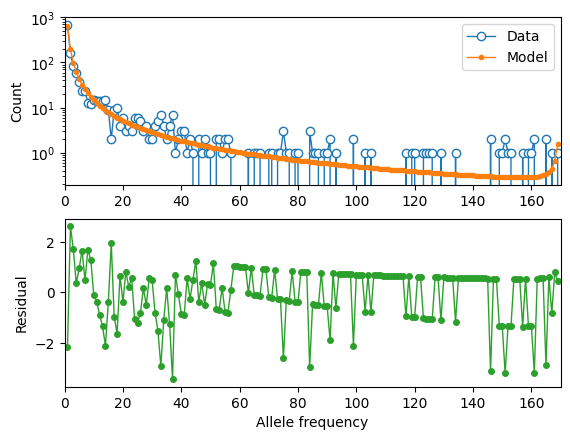
moments.Plotting.plot_1d_comp_multinom(model_lof, fs_lof, residual="linear")
optimal parameters:
shape: 0.5298
scale: 1601.8
anc misid: 0.0021
Log-likelihood: -237.79096099886442
And now comparing our results using the standard neutral model as the underlying demography:
print("Missense DFE:")
shape = opt_params_mis[0]
scale = opt_params_mis[1]
ss = [0, 1e-5, 1e-4, 1e-3, 1e-2]
for s0, s1 in zip(ss[:-1], ss[1:]):
    cdf0 = scipy.stats.gamma.cdf(2 * Ne * s0, shape, scale=scale)
    cdf1 = scipy.stats.gamma.cdf(2 * Ne * s1, shape, scale=scale)
    print(f"{s0} <= s < {s1}:", cdf1 - cdf0)
    if s1 == ss[-1]:
        print(f"s >= {s1}:", 1 - cdf1)

print()
print("LOF DFE:")
shape = opt_params_lof[0]
scale = opt_params_lof[1]
ss = [0, 1e-5, 1e-4, 1e-3, 1e-2]
for s0, s1 in zip(ss[:-1], ss[1:]):
    cdf0 = scipy.stats.gamma.cdf(2 * Ne * s0, shape, scale=scale)
    cdf1 = scipy.stats.gamma.cdf(2 * Ne * s1, shape, scale=scale)
    print(f"{s0} <= s < {s1}:", cdf1 - cdf0)
    if s1 == ss[-1]:
        print(f"s >= {s1}:", 1 - cdf1)
Missense DFE:
0 <= s < 1e-05: 0.10753022385488102
1e-05 <= s < 0.0001: 0.18776852548601913
0.0001 <= s < 0.001: 0.42679335393077866
0.001 <= s < 0.01: 0.27674764907249993
s >= 0.01: 0.0011602476558212338

LOF DFE:
0 <= s < 1e-05: 0.014239643653461635
1e-05 <= s < 0.0001: 0.03395207585847486
0.0001 <= s < 0.001: 0.11371870531196526
0.001 <= s < 0.01: 0.3451015784641346
s >= 0.01: 0.4929879967119637
These distributions look quite different - in particular, both the missense and LOF variants are inferred to be much more deleterious. This is because we did not account for population size expansions in it history, which leads to an excess of rare variants for each class of mutations, and the model over-compensates for the excess of rare variants by fitting a DFE that is more skewed toward larger selection coefficients.
References
Boyko, Adam R., et al. “Assessing the evolutionary impact of amino acid mutations in the human genome.” PLoS Genetics 4.5 (2008): e1000083.
Karczewski, Konrad J., et al. “The mutational constraint spectrum quantified from variation in 141,456 humans.” Nature 581.7809 (2020): 434-443.
Keightley, Peter D., and Adam Eyre-Walker. “Joint inference of the distribution of fitness effects of deleterious mutations and population demography based on nucleotide polymorphism frequencies.” Genetics 177.4 (2007): 2251-2261.
Kim, Bernard Y., Christian D. Huber, and Kirk E. Lohmueller. “Inference of the distribution of selection coefficients for new nonsynonymous mutations using large samples.” Genetics 206.1 (2017): 345-361.
Ragsdale, Aaron P., et al. “Triallelic population genomics for inferring correlated fitness effects of same site nonsynonymous mutations.” Genetics 203.1 (2016): 513-523.
1000 Genomes Project Consortium. “A global reference for human genetic variation.” Nature 526.7571 (2015): 68-74.